39 min to read
Understanding Quantum Computing - Next Generation Computing Technology
A comprehensive introduction to quantum computing principles and applications
Overview
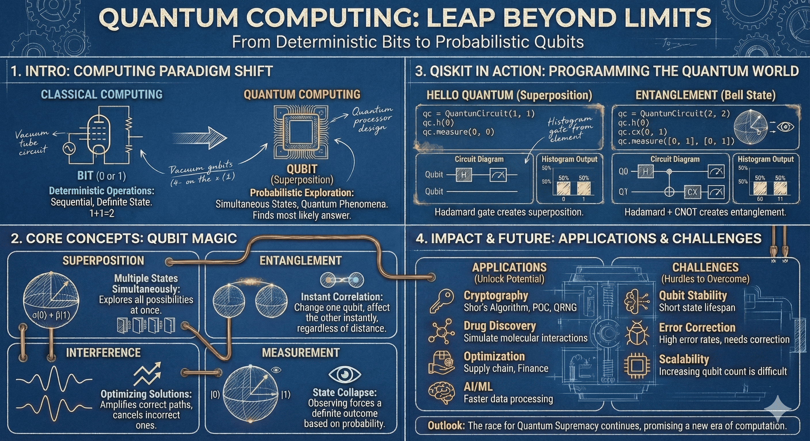
Quantum computing is a revolutionary computing paradigm that leverages quantum mechanical phenomena to perform calculations in ways fundamentally different from classical computers.
While traditional computers use bits (0 or 1) as the basic unit of information, quantum computers use quantum bits or “qubits” that can exist in multiple states simultaneously thanks to quantum superposition. This property, along with quantum entanglement and interference, allows quantum computers to solve certain complex problems exponentially faster than classical computers.
The theoretical foundations of quantum computing were established in the early 1980s by physicists Richard Feynman and Paul Benioff, who proposed using quantum mechanics for computation. In 1985, David Deutsch described the first universal quantum computer. The field gained momentum in 1994 when Peter Shor developed an algorithm that could efficiently factorize large numbers, demonstrating quantum computing's potential to break widely-used cryptographic systems.
The first experimental quantum computer with 2 qubits was demonstrated in 1998. Since then, companies like IBM, Google, and D-Wave have made significant advances, with Google claiming "quantum supremacy" in 2019 by performing a calculation that would be practically impossible for classical supercomputers.
Quantum Computing Explained
Definition
- Advanced computing paradigm using quantum mechanics principles
- Uses qubits instead of classical bits
- Exponentially faster for specific complex problems
- Leverages quantum properties like superposition and entanglement
The Three Quantum Principles
Superposition
Superposition is a fundamental quantum principle that allows qubits to exist in multiple states simultaneously.
Definition: Quantum state where a qubit can be both 0 and 1 at the same time
Mathematical Representation: |ψ⟩ = α|0⟩ + β|1⟩ where |α|² + |β|² = 1
Purpose: Enables quantum parallelism and exponential processing capability
In classical computing, a bit must be either 0 or 1. In quantum computing, superposition allows a qubit to exist as a combination of both states, with probabilities represented by complex numbers (amplitudes).
Basic Examples
# Creating a superposition state in Qiskit
from qiskit import QuantumCircuit

# Create a circuit with one qubit
qc = QuantumCircuit(1)

# Apply Hadamard gate to create superposition
qc.h(0)

# The qubit is now in superposition: 1/√2(|0⟩ + |1⟩)
Advanced Superposition Applications
# Creating different superposition states
qc = QuantumCircuit(1)

# Starting with |0⟩
qc.reset(0)

# Equal superposition
qc.h(0)  # 1/√2(|0⟩ + |1⟩)

# Biased superposition favoring |1⟩
qc.reset(0)
qc.ry(2.0, 0)  # Rotation around Y-axis changes amplitudes
Entanglement
Entanglement is a quantum correlation between qubits where the state of one qubit cannot be described independently of others.
Definition: Quantum phenomenon where qubits become correlated so that the state of one instantly influences others
Key Property: Non-local correlation regardless of physical distance
Purpose: Enables quantum communication and enhances quantum computing power
Einstein famously called entanglement “spooky action at a distance” because measuring one entangled qubit instantly determines the state of its entangled partner, even if they are physically separated.
Basic Examples
# Creating an entangled Bell pair in Qiskit
from qiskit import QuantumCircuit

# Create a circuit with two qubits
qc = QuantumCircuit(2)

# Put first qubit in superposition
qc.h(0)

# Entangle using CNOT gate
qc.cx(0, 1)

# Now qubits are in the Bell state: 1/√2(|00⟩ + |11⟩)
Advanced Entanglement Applications
# Creating different types of entangled states
qc = QuantumCircuit(2)

# Bell state Φ+ = 1/√2(|00⟩ + |11⟩)
qc.h(0)
qc.cx(0, 1)

# Bell state Φ- = 1/√2(|00⟩ - |11⟩)
qc.reset_all()
qc.h(0)
qc.cx(0, 1)
qc.z(1)

# Creating GHZ state with three qubits: 1/√2(|000⟩ + |111⟩)
qc = QuantumCircuit(3)
qc.h(0)
qc.cx(0, 1)
qc.cx(0, 2)
Quantum Interference
Quantum interference is a phenomenon where quantum amplitudes can enhance or cancel each other, directing computation toward desired outcomes.
Definition: Process where quantum probability amplitudes interact like waves
Key Feature: Both constructive and destructive interference are possible
Purpose: Amplifies correct solutions and reduces probability of wrong answers
Interference is what gives quantum algorithms their power. By carefully designing the sequence of operations, quantum developers can increase the probability of getting the correct answer.
Basic Examples
# Demonstrating interference in Qiskit
from qiskit import QuantumCircuit

# Create a circuit with one qubit
qc = QuantumCircuit(1)

# Apply Hadamard to get superposition
qc.h(0)  # 1/√2(|0⟩ + |1⟩)

# Apply Hadamard again
qc.h(0)  # Back to |0⟩ due to interference

# The second Hadamard causes interference that cancels out,
# deterministically returning the qubit to |0⟩
Advanced Interference Applications
# Quantum phase estimation uses interference to determine eigenvalues
from qiskit import QuantumCircuit

# Simplified quantum Fourier transform (QFT) example
qc = QuantumCircuit(3)
# Put all qubits in superposition
for qubit in range(3):
    qc.h(qubit)

# Add phase shifts
qc.p(3.14/2, 1)
qc.p(3.14/4, 2)

# Inverse QFT uses interference to extract phase information
# (simplified here)
qc.h(0)
qc.cx(0, 1)
qc.h(1)
qc.cx(0, 2)
qc.cx(1, 2)
qc.h(2)
Classical Computing vs Quantum Computing
| Aspect | Classical Computing | Quantum Computing |
|---|---|---|
| Basic Unit | Bit (0 or 1) | Qubit (superposition of 0 and 1) |
| Processing | Sequential or parallel | Simultaneous via superposition |
| State Representation | Single state at a time | Multiple states simultaneously |
| Speed | Efficient for general tasks | Exponentially faster for specific problems |
| Interconnectivity | No inherent correlation | Entanglement enables high connectivity |
| Output | Deterministic answer | Probabilistic result (highest probability outcome) |
| Error Susceptibility | Relatively robust | Highly sensitive to noise/decoherence |
Applications of Quantum Computing
Cryptography
- Shor’s algorithm can break existing encryption methods (e.g., RSA)
- Development of quantum-safe cryptography (Post-Quantum Cryptography)
- Quantum Key Distribution (QKD) for secure communication
Optimization Problems
- Supply chain management and logistics optimization
- Financial modeling and risk assessment
- Traffic flow optimization in smart cities
- Resource allocation in complex networks
Machine Learning
- Quantum machine learning can process large datasets much faster
- Quantum neural networks and quantum support vector machines
- Enhanced pattern recognition and data classification
- Potential breakthroughs in artificial intelligence
Drug Discovery and Material Science
- Simulating molecular interactions at the quantum level
- Accelerating new drug discovery and development
- Designing new materials with specific properties
- Understanding complex chemical reactions
Weather and Climate Modeling
- More accurate simulation of complex systems like weather patterns
- Climate dynamics modeling with higher precision
- Natural disaster prediction with improved accuracy
Quantum Simulation
- Simulating quantum systems impossible on classical computers
- Advancing fundamental physics and material science
- Studying quantum field theories and particle physics
- Exploring high-energy physics phenomena
Limitations and Challenges
Hardware Constraints
- Qubit decoherence (loss of quantum states due to interaction with environment)
- Extremely low operating temperatures (near absolute zero)
- Physical scaling challenges with increasing qubit numbers
- Quantum gate fidelity and measurement accuracy
Error Correction
- Quantum systems are highly prone to errors
- Effective quantum error correction is essential
- Error correction requires additional qubits
- Trade-off between computational power and error resilience
Scalability Issues
- Maintaining coherence and entanglement while increasing qubit count
- Physical and architectural limitations on qubit connectivity
- Manufacturing challenges for large-scale quantum processors
Cost Factors
- High production and maintenance costs
- Advanced technology and extreme cooling requirements
- Specialized infrastructure and expertise needed
- Significant research and development investment
Algorithm Development
- Limited number of quantum algorithms with proven advantages
- Complexity in designing efficient quantum algorithms
- Difficulty in translating classical problems to quantum formulations
- Early stage of quantum software development ecosystem
Deeper Understanding of Quantum Computing
Qubit vs. Bit: Visual Comparison
| Attribute | Bit (Classical) | Qubit (Quantum) |
|---|---|---|
| State | 0 or 1 (binary) | Superposition of 0 and 1 (probabilistic) |
| Visualization | Point on a line | Vector on a Bloch Sphere |
| Representation | 0, 1 | α|0⟩ + β|1⟩ (with complex coefficients) |
Qubits are commonly visualized using the Bloch Sphere representation, which shows the quantum state as a vector on a sphere.
Shor’s Algorithm
Shor’s algorithm is one of the most famous quantum algorithms, designed to factorize large numbers exponentially faster than the best-known classical algorithms.
- Current RSA encryption relies on the difficulty of factoring large numbers
- Shor’s algorithm poses a potential threat to RSA, ECC, and other cryptographic systems
- This has stimulated research in Post-Quantum Cryptography (PQC)
Note: Theoretically, Shor’s algorithm could break 2048-bit RSA in seconds with sufficient qubits.
Quantum Random Number Generation (QRNG)
While classical random number generation typically uses seed-based pseudo-random methods, Quantum Random Number Generators utilize the inherently unpredictable nature of quantum phenomena to produce true randomness.
- Leverages quantum entanglement and photon measurements for randomness
- Applications in security tokens, cryptographic key generation, gaming, and finance
- Some companies now offer QRNG APIs at the hardware level (e.g., ID Quantique)
Qiskit Example: Hello Quantum
IBM’s Qiskit framework allows for simulating and running actual quantum circuits. Here’s a simple example:
# Qiskit installation (first time only)
!pip install qiskit

# Basic imports
from qiskit import QuantumCircuit, Aer, execute
from qiskit.visualization import plot_histogram
import matplotlib.pyplot as plt

# Create quantum circuit
qc = QuantumCircuit(1, 1)   # 1 qubit, 1 measurement bit
qc.h(0)                     # Hadamard gate to create superposition
qc.measure(0, 0)            # Measure qubit 0 to classical bit 0

# Run on simulator
backend = Aer.get_backend('qasm_simulator')
job = execute(qc, backend=backend, shots=1000)
result = job.result()
counts = result.get_counts()

# Visualize output
print("Measurement results:", counts)
plot_histogram(counts)
plt.show()
- The execution results in a probability-based distribution like
{'0': 493, '1': 507}, demonstrating qubit superposition.
Key Quantum Gates and Operations
| Gate | Function | Qiskit Command | Description |
|---|---|---|---|
| Hadamard (H) | Creates superposition | qc.h(0) | |0⟩ → (1/√2)(|0⟩ + |1⟩) |
| Pauli-X (X) | NOT gate | qc.x(0) | |0⟩ ↔ |1⟩ |
| Pauli-Y (Y) | Complex rotation | qc.y(0) | Rotation with phase |
| Pauli-Z (Z) | Phase flip | qc.z(0) | Applies -1 phase to |1⟩ |
| CNOT (CX) | Controlled NOT (for Entanglement) | qc.cx(0, 1) | Flips target qubit if control qubit is 1 |
| Measure | State measurement | qc.measure(q, c) | Reads qubit into classical state |
Example: Creating Entangled Qubits
from qiskit import QuantumCircuit, Aer, execute
from qiskit.visualization import plot_histogram
import matplotlib.pyplot as plt

qc = QuantumCircuit(2, 2)
qc.h(0)         # Put first qubit in superposition
qc.cx(0, 1)     # Create entanglement
qc.measure([0, 1], [0, 1])

backend = Aer.get_backend('qasm_simulator')
result = execute(qc, backend, shots=1000).result()
counts = result.get_counts()

print("Entanglement measurement results:", counts)
plot_histogram(counts)
plt.show()
Expected result: {'00': ~500, '11': ~500}, demonstrating that qubits 0 and 1 are entangled.
Quantum Computing vs. Quantum Communication vs. Quantum Sensing
| Field | Description | Representative Technologies |
|---|---|---|
| Quantum Computing | Parallel computation using qubits | IBM Q, D-Wave, Google Sycamore |
| Quantum Communication | Entanglement-based secure communication | QKD, Quantum Internet |
| Quantum Sensing | Detecting minute signals using quantum states | Ultra-precise gravity measurement, medical imaging |
These three fields are technically complementary and have high application potential in defense, finance, space, energy, and various other industries.
Key Quantum Algorithms
Shor’s Algorithm
Shor’s algorithm is a quantum algorithm for finding the prime factors of an integer, exponentially faster than the best known classical algorithm.
# Simplified conceptual implementation of Shor's Algorithm
from qiskit import QuantumCircuit, Aer, execute
import numpy as np

def simplified_shor_factoring(N, a):
    """
    Very simplified conceptual representation of Shor's algorithm
    for factoring N using guess a (where 1 < a < N)
    """
    # Step 1: Create quantum circuit for period finding
    # (In a real implementation, this would be much more complex)
    qc = QuantumCircuit(8, 4)  # 8 qubits, 4 classical bits

    # Step 2: Initialize superposition
    for qubit in range(4):
        qc.h(qubit)

    # Step 3: Implement modular exponentiation
    # (This is a placeholder - actual implementation is complex)
    for i, qubit in enumerate(range(4)):
        if a % 2**i == 0:
            qc.cx(qubit, qubit+4)

    # Step 4: Quantum Fourier Transform
    for qubit in range(4):
        qc.h(qubit)

    # Step 5: Measure
    qc.measure(range(4), range(4))

    # Execute on simulator
    simulator = Aer.get_backend('qasm_simulator')
    result = execute(qc, simulator, shots=1000).result()
    counts = result.get_counts()

    # Step 6: Classical post-processing
    # Find the period r from measurement results (simplified)
    most_common = max(counts, key=counts.get)
    measured_value = int(most_common, 2)

    # Calculate factors (simplified)
    r = 2 * measured_value  # This is a simplification
    if r % 2 == 0:
        factor1 = np.gcd(a**(r//2) + 1, N)
        factor2 = np.gcd(a**(r//2) - 1, N)
        return factor1, factor2
    return "Failed to find factors"

# Example usage (conceptual only)
N = 15  # Number to factor
a = 7   # Coprime to N
print(simplified_shor_factoring(N, a))
Note: This is a highly simplified representation. The actual implementation requires dozens of qubits and complex quantum circuits.
Grover’s Algorithm
Grover’s algorithm provides a quadratic speedup for searching unsorted databases, finding an item in O(√N) steps compared to O(N) steps required classically.
# Simplified implementation of Grover's Algorithm
from qiskit import QuantumCircuit, Aer, execute
from qiskit.visualization import plot_histogram
import numpy as np
import matplotlib.pyplot as plt

def grover_search(marked_item, total_items):
    """
    Implementation of Grover's search for finding a marked item
    in an unsorted database.

    Args:
        marked_item: Item we're searching for (as an integer)
        total_items: Total number of items in database

    Returns:
        Quantum circuit with Grover's algorithm
    """
    # Calculate required qubits
    n = int(np.ceil(np.log2(total_items)))

    # Create quantum circuit
    qc = QuantumCircuit(n, n)

    # Step 1: Initialize superposition
    qc.h(range(n))

    # Number of iterations (optimal for single marked item)
    iterations = int(np.pi/4 * np.sqrt(total_items))

    for _ in range(iterations):
        # Step 2: Oracle - mark the solution
        # (In a real implementation, this would encode the search problem)
        # Here we just flip the phase of the marked item state
        marked_binary = format(marked_item, f'0{n}b')
        qc.barrier()

        # Implement simple oracle by applying Z to marked state
        # (For simplicity, we use X gates to flip bits where marked_binary has '0')
        for qubit, bit in enumerate(reversed(marked_binary)):
            if bit == '0':
                qc.x(qubit)

        # Multi-controlled Z gate (simplification)
        if n > 1:
            qc.h(n-1)
            qc.mcx(list(range(n-1)), n-1)
            qc.h(n-1)
        else:
            qc.z(0)

        # Flip bits back
        for qubit, bit in enumerate(reversed(marked_binary)):
            if bit == '0':
                qc.x(qubit)

        # Step 3: Diffusion operator (amplification)
        qc.barrier()
        qc.h(range(n))
        qc.x(range(n))

        # Apply controlled-Z
        if n > 1:
            qc.h(n-1)
            qc.mcx(list(range(n-1)), n-1)
            qc.h(n-1)
        else:
            qc.z(0)

        qc.x(range(n))
        qc.h(range(n))

    # Measure the result
    qc.measure(range(n), range(n))

    return qc

# Example usage
marked_item = 6  # The item we're searching for
total_items = 8  # Total items in database

# Create and run the circuit
qc = grover_search(marked_item, total_items)
simulator = Aer.get_backend('qasm_simulator')
result = execute(qc, simulator, shots=1024).result()
counts = result.get_counts()

# Display results
print(f"Searching for item {marked_item} among {total_items} items:")
print(f"Measurement results: {counts}")
most_common = max(counts, key=counts.get)
print(f"Found item: {int(most_common, 2)}")
Quantum Fourier Transform (QFT)
The Quantum Fourier Transform is a critical component of many quantum algorithms, including Shor’s algorithm and quantum phase estimation.
# Implementation of Quantum Fourier Transform
from qiskit import QuantumCircuit
import numpy as np

def qft_rotations(circuit, n):
    """Apply QFT rotations to all qubits in circuit"""
    if n == 0:
        return circuit
    n -= 1
    circuit.h(n)
    for qubit in range(n):
        circuit.cp(np.pi/2**(n-qubit), qubit, n)
    return qft_rotations(circuit, n)

def swap_registers(circuit, n):
    """Swap qubits for the correct output order"""
    for qubit in range(n//2):
        circuit.swap(qubit, n-qubit-1)
    return circuit

def qft(circuit, n):
    """Quantum Fourier Transform on n qubits"""
    qft_rotations(circuit, n)
    swap_registers(circuit, n)
    return circuit

# Example: 4-qubit QFT circuit
qc = QuantumCircuit(4)

# Prepare some non-trivial state
qc.x(0)
qc.x(2)

# Apply QFT
qft(qc, 4)

print("QFT Circuit:")
print(qc)
Quantum Hardware and Implementation
Types of Quantum Computers
| Type | Description | Advantages/Disadvantages |
|---|---|---|
| Superconducting | Uses superconducting circuits cooled to near absolute zero to create qubits | Advantages: Scalable, fast gate operations Disadvantages: Very low temperature requirements, short coherence time |
| Trapped Ion | Uses electromagnetic fields to trap ions as qubits | Advantages: Long coherence time, high fidelity gates Disadvantages: Slower gate operations, scaling challenges |
| Photonic | Uses photons (particles of light) as qubits | Advantages: Room temperature operation, natural for communication Disadvantages: Probabilistic gates, photon loss |
| Quantum Annealing | Special-purpose quantum computers optimized for specific optimization problems | Advantages: More qubits available now, specialized for optimization Disadvantages: Limited to specific problem types, not universal |
| Topological | Theoretical approach using topological properties for error-resistant qubits | Advantages: Inherent error protection, potentially stable Disadvantages: Still largely theoretical, complex to implement |
Quantum Programming Frameworks
| Framework | Developer | Key Features | Best For |
|---|---|---|---|
| Qiskit | IBM | Comprehensive toolset, access to IBM quantum hardware, rich visualization tools | General-purpose quantum programming, circuit design, algorithm development |
| Cirq | Low-level control, focus on NISQ era hardware, integration with TensorFlow | Near-term quantum algorithms, hardware-specific optimization | |
| PennyLane | Xanadu | Quantum machine learning focus, automatic differentiation, hybrid quantum-classical | Quantum ML, variational quantum algorithms, optimization |
| Q# | Microsoft | Integration with Visual Studio, high-level language features, quantum simulation | Enterprise development, scalable quantum solutions |
| Forest (pyQuil) | Rigetti | Quil assembly language, Quantum Virtual Machine, hybrid computing | Low-level quantum programming, access to Rigetti hardware |
Troubleshooting Common Issues in Quantum Computing
Addressing Quantum Noise
# Techniques for addressing quantum noise
from qiskit import QuantumCircuit
from qiskit.ignis.mitigation.measurement import complete_meas_cal, CompleteMeasFitter

def measurement_error_mitigation():
    """
    Demonstrate measurement error mitigation technique
    """
    # Create a calibration circuit
    qc = QuantumCircuit(2)

    # Generate calibration circuits
    meas_calibs, state_labels = complete_meas_cal(qubit_list=[0, 1], qr=qc.qregs[0])

    # Execute calibration circuits
    # In a real scenario, you would run these on actual quantum hardware
    from qiskit import Aer, execute
    simulator = Aer.get_backend('qasm_simulator')
    # Add artificial measurement error
    from qiskit.providers.aer.noise import NoiseModel
    noise_model = NoiseModel()
    noise_model.add_readout_error([[0.95, 0.05], [0.05, 0.95]], [0])
    noise_model.add_readout_error([[0.93, 0.07], [0.07, 0.93]], [1])

    cal_results = execute(meas_calibs, simulator,
                         shots=1000,
                         noise_model=noise_model).result()

    # Build the measurement error mitigator
    meas_fitter = CompleteMeasFitter(cal_results, state_labels)

    # Create a test circuit
    test_qc = QuantumCircuit(2, 2)
    test_qc.h(0)
    test_qc.cx(0, 1)
    test_qc.measure([0,1], [0,1])

    # Execute with noise
    test_results = execute(test_qc, simulator,
                          shots=1000,
                          noise_model=noise_model).result()
    test_counts = test_results.get_counts()

    # Apply measurement error mitigation
    mitigated_counts = meas_fitter.filter.apply(test_counts)

    print("Original noisy counts:", test_counts)
    print("Mitigated counts:", mitigated_counts)

    return mitigated_counts

# Run measurement error mitigation example
# measurement_error_mitigation()
Debugging Quantum Circuits
# Techniques for debugging quantum circuits
from qiskit import QuantumCircuit, Aer, transpile
from qiskit.visualization import plot_state_city, plot_bloch_multivector

def quantum_circuit_debugging():
    """
    Demonstrate debugging techniques for quantum circuits
    """
    # Create a circuit with a bug
    qc = QuantumCircuit(2)
    qc.h(0)
    # Intentional "bug": missing CNOT gate for entanglement
    # qc.cx(0, 1)  # This line is commented out to create a bug

    # Debug technique 1: Statevector simulation
    simulator = Aer.get_backend('statevector_simulator')
    job = simulator.run(transpile(qc, simulator))
    result = job.result()
    statevector = result.get_statevector()

    print("Statevector after circuit execution:")
    print(statevector)
    # The statevector shows no entanglement (|+0⟩ state instead of Bell state)

    # Debug technique 2: Density matrix visualization
    # plot_state_city(statevector)

    # Debug technique 3: Bloch sphere visualization
    # plot_bloch_multivector(statevector)

    # Debug technique 4: Circuit transpilation inspection
    transpiled_qc = transpile(qc, basis_gates=['u1', 'u2', 'u3', 'cx'])
    print("Transpiled circuit operations:")
    print(transpiled_qc.count_ops())

    # Debug technique 5: Step-by-step execution
    step_qc = QuantumCircuit(2)

    # Step 1: Apply H gate and check state
    step_qc.h(0)
    step_result = simulator.run(transpile(step_qc, simulator)).result()
    step_state = step_result.get_statevector()
    print("State after H gate:", step_state)

    # Step 2: Now add the missing CNOT and check again
    step_qc.cx(0, 1)
    step_result = simulator.run(transpile(step_qc, simulator)).result()
    step_state = step_result.get_statevector()
    print("State after CNOT gate:", step_state)

    # Fix the original circuit
    fixed_qc = QuantumCircuit(2)
    fixed_qc.h(0)
    fixed_qc.cx(0, 1)  # Bug fixed by adding CNOT

    # Verify the fix
    fixed_result = simulator.run(transpile(fixed_qc, simulator)).result()
    fixed_state = fixed_result.get_statevector()
    print("Fixed circuit state:", fixed_state)

    return fixed_qc

# Run quantum debugging example
# quantum_circuit_debugging()
Common Quantum Computing Errors
| Error Type | Description | Mitigation Strategies |
|---|---|---|
| Decoherence | Loss of quantum information due to environment interaction | Reduce circuit depth, use faster gates, improve physical isolation, error correction codes |
| Gate Errors | Imperfect implementation of quantum operations | Gate calibration, robust gate design, dynamical decoupling, composite pulses |
| Readout Errors | Mistakes in measuring qubit states | Measurement error mitigation, readout calibration, repeated measurements |
| Crosstalk | Unintended interaction between qubits | Improved hardware design, pulse scheduling, crosstalk-aware compilation |
| Leakage | Qubits leaving computational subspace | Leakage reduction units, careful pulse design, improved qubit isolation |
| Transpilation Errors | Suboptimal translation of abstract circuit to hardware | Custom transpilation passes, hardware-aware compilation, circuit optimization |
Future Prospects
Quantum Computing Timeline
| Timeframe | Expected Developments | Potential Applications |
|---|---|---|
| Near-term (1-3 years) | Noisy Intermediate-Scale Quantum (NISQ) computers with 100-1000 qubits, limited error correction | Optimization problems, materials science simulations, limited quantum machine learning, financial modeling |
| Mid-term (3-10 years) | Fault-tolerant logical qubits, early error correction, specialized quantum advantages | Quantum chemistry simulations, drug discovery, advanced optimization, enhanced machine learning, select cryptographic applications |
| Long-term (10+ years) | Fully error-corrected quantum computers, millions of logical qubits, quantum memory | Breaking classical encryption, large-scale simulations, quantum AI, quantum network communications, quantum internet |
Emerging Applications
- Quantum Internet: Secure communication networks using quantum entanglement and teleportation
- Quantum Sensors: Ultra-precise measurements for navigation, medical imaging, and gravitational wave detection
- Quantum AI: New paradigms for machine learning leveraging quantum phenomena
- Quantum Batteries: Energy storage technologies based on quantum coherence
- Quantum Money: Unforgeable currency based on quantum no-cloning principles
Key Points
-
Quantum Paradigms
- Superposition: Qubits exist in multiple states
- Entanglement: Correlation between qubits
- Interference: Wave-like interaction of probabilities -
Key Algorithms
- Shor's: Factoring large numbers
- Grover's: Searching unstructured databases
- VQE: Quantum chemistry simulations
- QFT: Foundation for many quantum algorithms -
Practical Impact
- Cybersecurity transformation
- Acceleration of material and drug discovery
- Complex optimization solutions
- New paradigms in machine learning
As of 2025, the leading quantum computing platforms include:
- IBM Quantum: Up to 433 qubits (Eagle processor), superconducting technology, accessible via cloud
- Google Quantum AI: 72 qubits (Bristlecone), focusing on quantum supremacy demonstrations
- D-Wave: Over 5000 qubits, but using quantum annealing (specialized for optimization problems)
- IonQ: 32 qubits with very high fidelity using trapped ion technology
- Rigetti: 80+ qubits using superconducting technology
While qubit count is often highlighted, the quality of qubits (measured by coherence time, gate fidelity, and connectivity) is equally important for determining a quantum computer's capabilities.
The quantum computing technology stack consists of multiple layers:
- Physical Layer: Qubits and control hardware
- Control Layer: Pulse sequences and calibration
- Gate Layer: Quantum gates and error correction
- Algorithm Layer: Quantum circuits and subroutines
- Application Layer: Industry-specific quantum solutions
Different quantum computing companies focus on different parts of this stack, with full-stack providers like IBM and Google covering everything from hardware to software.
Practical Use Cases
Quantum Cryptography
# Simplified Quantum Key Distribution (BB84 protocol)
from qiskit import QuantumCircuit, Aer, execute
import numpy as np
import random

def bb84_protocol(n_bits=8):
    """
    Simulate the BB84 quantum key distribution protocol

    Args:
        n_bits: Number of bits in the key

    Returns:
        Shared secret key
    """
    # Step 1: Alice prepares qubits in random bases with random values
    alice_bits = [random.randint(0, 1) for _ in range(n_bits)]
    alice_bases = [random.randint(0, 1) for _ in range(n_bits)]  # 0=Z basis, 1=X basis

    # Create circuits for each qubit
    circuits = []
    for bit, basis in zip(alice_bits, alice_bases):
        qc = QuantumCircuit(1, 1)

        # Prepare qubit according to bit value
        if bit == 1:
            qc.x(0)

        # Apply Hadamard if using X basis
        if basis == 1:
            qc.h(0)

        circuits.append(qc)

    # Step 2: Bob measures in random bases
    bob_bases = [random.randint(0, 1) for _ in range(n_bits)]

    # Bob's measurement
    bob_results = []
    for i, (qc, basis) in enumerate(zip(circuits, bob_bases)):
        # If Bob uses X basis, apply Hadamard before measurement
        if basis == 1:
            qc.h(0)

        qc.measure(0, 0)

        # Simulate the measurement
        simulator = Aer.get_backend('qasm_simulator')
        result = execute(qc, simulator, shots=1).result()
        counts = result.get_counts()
        measured_bit = int(list(counts.keys())[0])
        bob_results.append(measured_bit)

    # Step 3: Basis reconciliation (public discussion)
    matching_bases = []
    for i in range(n_bits):
        if alice_bases[i] == bob_bases[i]:
            matching_bases.append(i)

    # Step 4: Extract the key from positions with matching bases
    secret_key = [alice_bits[i] for i in matching_bases]

    # Print the protocol steps
    print(f"Alice's random bits: {alice_bits}")
    print(f"Alice's random bases: {['Z' if b==0 else 'X' for b in alice_bases]}")
    print(f"Bob's random bases: {['Z' if b==0 else 'X' for b in bob_bases]}")
    print(f"Bob's measured bits: {bob_results}")
    print(f"Positions with matching bases: {matching_bases}")
    print(f"Final shared secret key: {secret_key}")

    return secret_key

# Run the BB84 protocol simulation
bb84_protocol(16)
Quantum Chemistry Simulation
Quantum Computing Milestones
Common Patterns and Best Practices
Quantum Circuit Design
# Best practices for quantum circuit design
from qiskit import QuantumCircuit

# Good practice: Minimize circuit depth
qc = QuantumCircuit(3)
# Instead of multiple sequential gates:
qc.h([0, 1, 2])  # Apply H gates in parallel

# Good practice: Use barriers for clarity
qc.barrier()

# Good practice: Use specialized composite gates
# instead of decomposing into many basic gates
qc.ccx(0, 1, 2)  # Toffoli gate
Error Mitigation Techniques
# Example of zero-noise extrapolation
from qiskit import QuantumCircuit, transpile, Aer
from qiskit.providers.aer.noise import NoiseModel

# Create a simple circuit
qc = QuantumCircuit(2, 2)
qc.h(0)
qc.cx(0, 1)
qc.measure([0, 1], [0, 1])

# Define noise scaling factors
scale_factors = [1.0, 2.0, 3.0]
results = []

# Create a simple noise model
noise_model = NoiseModel()
# Add depolarizing error to gates (simplified)
error_rate = 0.01
noise_model.add_all_qubit_quantum_error(error_rate, ['h', 'cx'])

# Run for each noise scale
for scale in scale_factors:
    # Scale the noise (simplified)
    scaled_model = NoiseModel()
    scaled_model.add_all_qubit_quantum_error(error_rate * scale, ['h', 'cx'])

    # Run the circuit
    simulator = Aer.get_backend('qasm_simulator')
    result = simulator.run(transpile(qc, simulator),
                          noise_model=scaled_model,
                          shots=1000).result()
    counts = result.get_counts()

    # Record expectation value (probability of |00⟩)
    p00 = counts.get('00', 0) / 1000
    results.append(p00)

# Extrapolate to zero noise (simplified linear extrapolation)
import numpy as np
from scipy.optimize import curve_fit

def linear_model(x, a, b):
    return a * x + b

# Fit and extrapolate
popt, _ = curve_fit(linear_model, scale_factors, results)
zero_noise_result = linear_model(0, *popt)

print(f"Noisy results: {results}")
print(f"Extrapolated zero-noise result: {zero_noise_result}")
Conclusion
Quantum computing represents a fundamental shift in computational paradigms. While classical computers process information in deterministic binary states, quantum computers harness the probabilistic nature of quantum mechanics to solve problems in novel ways.
The journey from theoretical concept to practical technology has accelerated dramatically in recent years. Major technology companies and startups have moved from simple proof-of-concept devices to systems with hundreds of qubits that can perform useful, if limited, computations.
Despite significant hardware and theoretical challenges, the field is progressing rapidly. Error correction techniques, more stable qubit designs, and advances in quantum algorithms are gradually addressing current limitations.
As quantum computers continue to evolve from noisy, experimental systems to fault-tolerant, practical tools, we can expect transformative impacts across industries - from cybersecurity and pharmaceutical development to financial modeling and artificial intelligence.
The quantum computing revolution is not just about faster computers - it represents a fundamentally new way of processing information that will enable us to solve problems previously considered intractable, opening new frontiers in science and technology.

Comments