9 min to read
Load Average in top Command - What It Really Means
Understanding system load metrics beyond CPU usage
Overview
Load Average is one of the most commonly monitored metrics in Linux systems administration and performance analysis. It provides a high-level view of system resource utilization over time, serving as an early warning system for potential performance bottlenecks. When you run commands like top, uptime, or htop, you’ll see three numbers representing the 1, 5, and 15-minute load averages.
However, load average is also one of the most misunderstood metrics. Many system administrators erroneously equate it directly with CPU usage, leading to incorrect interpretations like “a load of 2.0 means the CPU is 200% utilized” or “any load above 1.0 indicates an overloaded system.”
The reality is more nuanced – load average combines several factors into a single metric that reflects the “pressure” on your system. Understanding this metric correctly is essential for effective system monitoring, capacity planning, and troubleshooting in production environments.
The concept of load average originated in the early Unix systems of the 1970s. It was designed to provide a simple measure of system busyness that could be understood at a glance and compared over time.
The original Unix implementation only counted processes in the run queue (either running or waiting for CPU time). However, Linux later expanded this definition in the early 1990s to include processes in uninterruptible sleep states (D state), primarily those waiting for I/O operations to complete.
This difference in implementation explains why the interpretation of load average varies between Unix-like systems, and why Linux load averages tend to be higher than those on systems like FreeBSD or macOS for equivalent workloads. The Linux kernel developer Matthias Urlichs described the inclusion of I/O wait in load average as "the most unlucky design decision in the history of Unix" due to the confusion it causes, though others argue it provides a more complete picture of system resource contention.
What is Load Average?
Load Average is a measurement of system demand over time, expressed as the average number of processes that are either:
- Running (using CPU)
- Runnable (waiting for CPU time)
- Uninterruptible Sleep (waiting for I/O operations, typically disk I/O)
Think of it as a measure of the “queue length” of processes demanding system resources. If you have a load average of 1.0, it means that over the measured time period, there was, on average, exactly one process active or waiting for resources at any given time.
The three load average numbers you typically see represent averages over different time periods:
- 1-minute average: Recent system activity
- 5-minute average: Intermediate-term trend
- 15-minute average: Long-term system behavior
Imagine a single checkout lane at a grocery store:
- A load of 1.0 means there's exactly one customer being served at all times.
- A load of 0.5 means the checkout lane is idle half the time.
- A load of 2.0 means there's one customer being served and one waiting in line, on average.
- A load of 10.0 means there's one customer being served and nine waiting in line, on average.
Now imagine you have a store with 4 checkout lanes (like a 4-core CPU):
- A load of 4.0 means all checkout lanes are busy, but no one is waiting.
- A load below 4.0 means some lanes are occasionally idle.
- A load above 4.0 means customers are waiting (indicating potential performance issues).
How Load Average is Calculated
Load Average isn’t a simple arithmetic mean but an Exponential Moving Average. This means recent data carries more weight in the calculation, making it more responsive to changes.
- 1-minute average → More sensitive to recent changes
- 15-minute average → Better for observing long-term trends
This calculation method makes it easy to compare sudden load increases with sustained load conditions.
Components of Load Average
Load Average is not simply CPU usage, but is calculated based on the number of processes in the following states:
| State | Included | Description |
|---|---|---|
| Running | Yes | Processes currently executing |
| Runnable | Yes | Processes waiting for CPU allocation |
| I/O Wait | Yes (Linux only) | Processes waiting for I/O (e.g., disk/network) |
| Sleeping / Idle | No | Processes not doing any work |
In essence, Load Average represents how many processes “are currently using or waiting to use the CPU.”
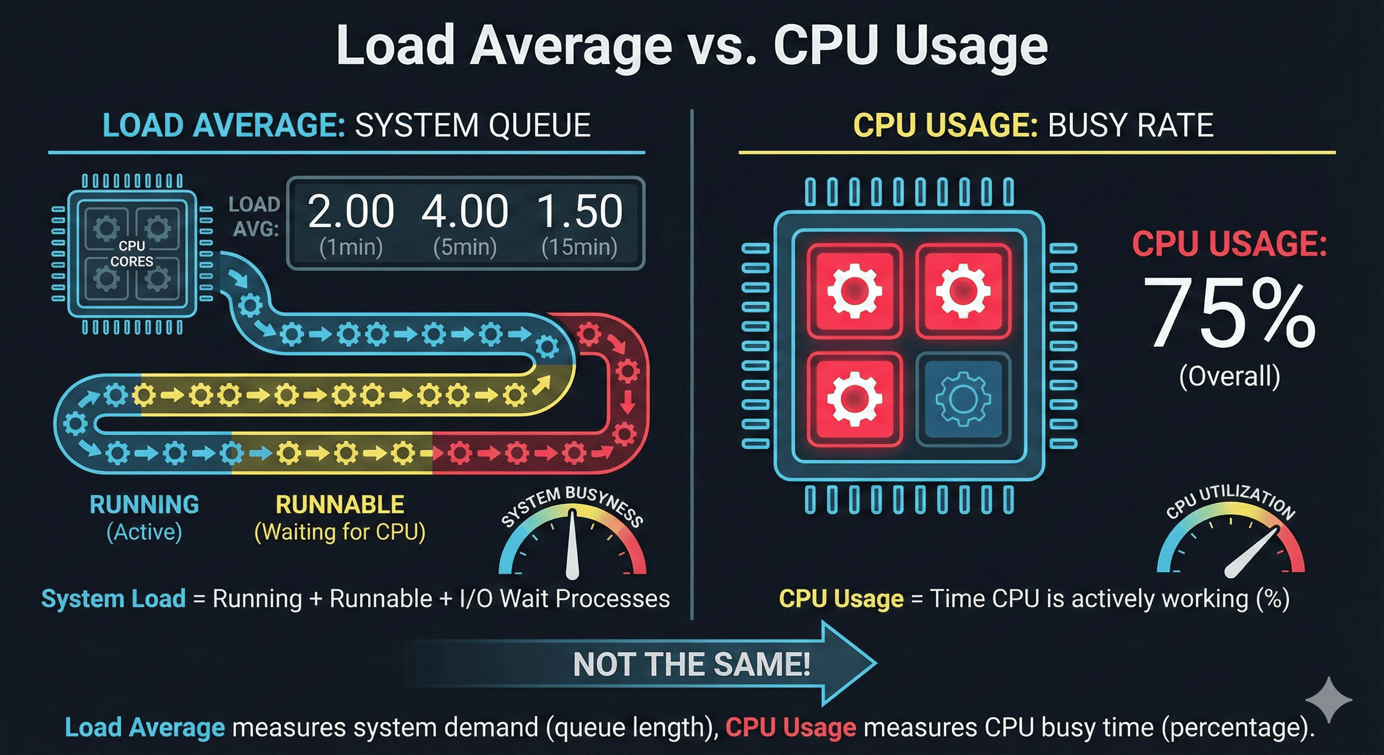
Load Average vs CPU Usage
| Aspect | Load Average | CPU Usage |
|---|---|---|
| Meaning | Overall system workload | Percentage of time CPU is actually working |
| Components | Running + waiting processes | CPU time (%) |
| Unit | Number of processes | Percentage (%) |
| Example | Load 2.00 = 2 processes running simultaneously | CPU usage 80% = CPU busy 80% of the time |
Common Misconceptions
- “Load Average is CPU usage” → ❌ No! It’s the number of processes (including waiting ones)
- “Load of 2 means CPU is used at 200%” → ❌ Must consider the number of CPU cores
- “High load means poor server performance” → ❌ Could be due to I/O bottlenecks
Interpreting Load Average Values
How you interpret load average depends on your system’s CPU count. The common rule of thumb is:
- Load average ≈ number of CPUs: The system is fully utilized but not overloaded
- Load average < number of CPUs: The system has spare capacity
- Load average > number of CPUs: The system is potentially overloaded
Consider a 4-core server with these load averages: 2.34, 3.45, 4.56
- 1-minute (2.34): The system is at ~58% capacity (2.34/4). There's still headroom.
- 5-minute (3.45): The system is at ~86% capacity (3.45/4). Getting close to full utilization.
- 15-minute (4.56): The system is at ~114% capacity (4.56/4). The server has been overloaded for some time.
This pattern suggests:
- The system was overloaded (15-min average > 4)
- The situation is improving (1-min average < 5-min average < 15-min average)
- No immediate action may be needed, but monitoring should continue
If the pattern were reversed (1-min > 5-min > 15-min), it would indicate a worsening situation requiring prompt investigation.
Is High Load Always Bad?
Not necessarily. Consider these factors:
- Duration: Brief spikes are normal during batch operations
- Composition: CPU-bound load differs from I/O-bound load
- System Response: If the system remains responsive despite high load, it may be acceptable
- Expected Patterns: Some applications naturally create periodic high load
Interpretation Tips for Production
Checkpoints
- Sudden increase: If 1-minute average is higher than 5/15-minute averages, load has increased rapidly
- Consistent high load: If 15-minute average is consistently high, there’s a persistent bottleneck
- I/O wait inclusion: Determine if the bottleneck is disk-related or CPU-related (use iostat, vmstat)
Monitoring Examples
- Real-time monitoring available in top, uptime, htop, grafana, prometheus.node_exporter
- Prometheus query example:
node_load1 / count(node_cpu_seconds_total{mode="idle"})
How is Load Average Used in Kubernetes?
In K8s node autoscaling, custom metrics based on Load Average can be applied alongside CPU usage criteria. Example: With Prometheus + KEDA combination, node_load1 / core count can be used as a criterion for scaling out.
Practical Examples
$ top
load average: 1.5, 1.2, 1.0
- On a 4-core system? → Plenty of capacity
- On a 1-core system? → Already experiencing wait bottlenecks
$ top
load average: 5.0, 4.9, 5.1
- On a 2-core system? → Overloaded; check queries/batch jobs/IO
Troubleshooting High Load Average
When load average exceeds your CPU count for extended periods, here are some commands to help diagnose the issue:
# View top processes by CPU usage
top

# Sort by memory usage in top
# Press Shift+M while top is running

# View processes in tree format
pstree -p

# Check I/O operations
iostat -x 1

# View memory usage
free -h

# Check for processes in uninterruptible sleep (D state)
ps aux | grep -w D

# Check system activity reports over time
sar -q
The most common causes of high load average include:
- CPU-bound processes: Computationally intensive tasks consuming CPU cycles
- Memory pressure: Excessive swapping due to memory shortage
- I/O bottlenecks: Slow disk operations causing processes to wait
- Resource contention: Multiple processes competing for the same resources
- Runaway processes: Processes in infinite loops or with memory leaks
Conclusion: “Not CPU Usage, But Length of the System’s Queue”
Load Average is not simply CPU usage, but an indirect indicator of system load showing ‘how many processes were waiting for CPU or resource allocation.’
Therefore, rather than simply evaluating it as “high/low”:
- Compare with CPU core count → If Load Average is consistently higher than the CPU Core count, there may be a bottleneck
- Analyze time trends → Looking at the flow between 1/5/15-minute averages helps determine if the issue is ‘sudden’ vs ‘persistent’
- Combine with iowait analysis → Accurately distinguish between CPU bottlenecks and disk bottlenecks to take appropriate action
In practice, it’s best to comprehensively identify bottlenecks by looking at CPU usage + Load Average + iowait together.
Practical Tips
- Short-term spikes can be ignored, but high loads persisting beyond the 15-minute average should be investigated
- When I/O wait is also high, disk delays, NFS bottlenecks, or backup operations may be suspects
- Visualizing trends with Prometheus, Grafana, etc. makes it much easier to identify spikes and their causes
In conclusion, Load Average is not just a number but closer to the “breathing of your system.” Being able to read this metric correctly gives you the ability to detect problem signs early and prevent failures.


Comments