23 min to read
Supervised vs Unsupervised Learning: Understanding ML Fundamentals with Fruit Classification
From fruit sorting to advanced algorithms - A complete guide to machine learning paradigms
Table of Contents
- Overview
- Supervised vs Unsupervised Learning
- Similarity vs Compatibility
- Hands-on Python Examples
- Advanced Case Studies
- Why Both Approaches Matter
- UCI Machine Learning Repository
- Conclusion
- References
Overview
When starting with machine learning, one of the most common questions is: “What’s the difference between supervised and unsupervised learning?” This comprehensive guide uses intuitive fruit classification examples and real Python implementations to explain the core concepts that form the foundation of modern AI systems.
Through practical examples involving fruit classification and the famous Iris dataset, we’ll explore:
- Supervised Learning: Classification and prediction with labeled data
- Unsupervised Learning: Pattern discovery without ground truth labels
- Similarity: Measuring how alike two data points are
- Compatibility: Evaluating how well items work together
You’ll gain hands-on experience with algorithms like DecisionTree, SVM, KNN, LogisticRegression for classification, and KMeans clustering with similarity analysis using real Python code.
Supervised vs Unsupervised Learning
Supervised Learning - “Learning with Answers”
Definition
“This fruit is an apple” → Learning from data where the correct answers (labels) are provided
| Characteristic | Description |
|---|---|
| Input | Fruit features: color, size, sweetness, etc. |
| Output | Labels (e.g., apple, banana, grape) |
| Goal | Learn to predict correct labels for new input data |
| Example | Fruit image → Apple/Banana/Grape prediction |
Example:
Input: [color=red, size=small, sweetness=high]
Output: Apple (label)
Unsupervised Learning - “Finding Patterns Without Answers”
Definition
“These fruits look similar, they might belong to the same group!” → Discovering data structure without ground truth labels
| Characteristic | Description |
|---|---|
| Input | Fruit features: color, size, sweetness, etc. |
| Output | None (clusters/groups without predefined labels) |
| Goal | Group similar data points or extract meaningful features |
| Example | Automatically cluster fruits by color/size similarity |
Example:
Input: Various fruit feature data
Output: Cluster 1 = Apple-like group, Cluster 2 = Banana-like group
Similarity vs Compatibility
While similarity and compatibility may seem related, they serve different purposes in machine learning applications.
Similarity
Core Question
“How alike are these two objects?” → Measuring distance or resemblance between data points
| Characteristic | Description |
|---|---|
| Core Question | How similar are they? |
| Mathematical Expression | Cosine Similarity, Euclidean Distance, etc. |
| Use Cases | Recommendation systems, clustering, image search |
Example:
Apple vs Pear color/sweetness/size difference → Distance calculation
Distance 0 = Nearly identical fruits
Compatibility
Core Question
“How well do these items work together?” → Evaluating the quality of combinations
| Characteristic | Description |
|---|---|
| Core Question | How well do they work together? |
| Mathematical Expression | Score-based (interaction models, co-occurrence) |
| Use Cases | Matching systems, product recommendations, recipe pairing |
Example:
Apple + Honey combination score = 9.1
Apple + Soy sauce combination score = 2.3
Summary: ML Concepts with Fruit Examples
| Concept | Description | Example |
|---|---|---|
| Supervised Learning | Learning from labeled examples | Fruit photo → Apple prediction |
| Unsupervised Learning | Finding groups without labels | Grouping similar fruits together |
| Similarity | How alike are they? | Apple vs Pear comparison |
| Compatibility | How well do they work together? | Apple + Honey pairing |
Hands-on Python Examples
Now let’s implement supervised and unsupervised learning with actual Python code. Follow along with the practical examples below.
🚀 Complete Code Repository
� ML Basics - Supervised vs Unsupervised Learning
Complete guide from machine learning fundamentals to hands-on practice
What’s included:
- 📓 Interactive Jupyter Notebooks
- 📊 Real-world Sample Datasets
- 🐍 Well-documented Python Examples
- 📚 Step-by-step Implementation Guide
- 🔬 Comparison Analysis & Visualizations
� Prerequisites
Before diving into the examples, make sure you have the following setup ready:
Setup: Virtual Environment and Dependencies
Recommended Setup
Create a virtual environment to avoid package conflicts and ensure reproducible results.
# Create and activate virtual environment
python3 -m venv ml_env
source ml_env/bin/activate  # Windows: ml_env\Scripts\activate

# Install required packages
pip3 install scikit-learn numpy matplotlib pandas
Example 1: Fruit Classification with Scikit-Learn
This example demonstrates both supervised and unsupervised learning approaches using synthetic fruit data with features like color, size, and sweetness.
# supervised_vs_unsupervised.py
from sklearn.tree import DecisionTreeClassifier
from sklearn.cluster import KMeans
from sklearn.metrics.pairwise import cosine_similarity
import numpy as np
import matplotlib.pyplot as plt
# Configure font for better visualization
plt.rcParams['font.family'] = 'DejaVu Sans'
plt.rcParams['axes.unicode_minus'] = False
# -----------------------
# Supervised Learning: Fruit Classification
# -----------------------
print("📘 Supervised Learning - Decision Tree Fruit Prediction")
# Fruit features: [color, size, sweetness]
X = [[1, 1, 9], [1, 2, 10], [3, 4, 3], [2, 4, 4], [4, 1, 8]]
y = [0, 0, 1, 1, 2] # 0:apple, 1:banana, 2:grape
clf = DecisionTreeClassifier(random_state=42)
clf.fit(X, y)
# Predict new fruit
prediction = clf.predict([[1, 1, 10]])
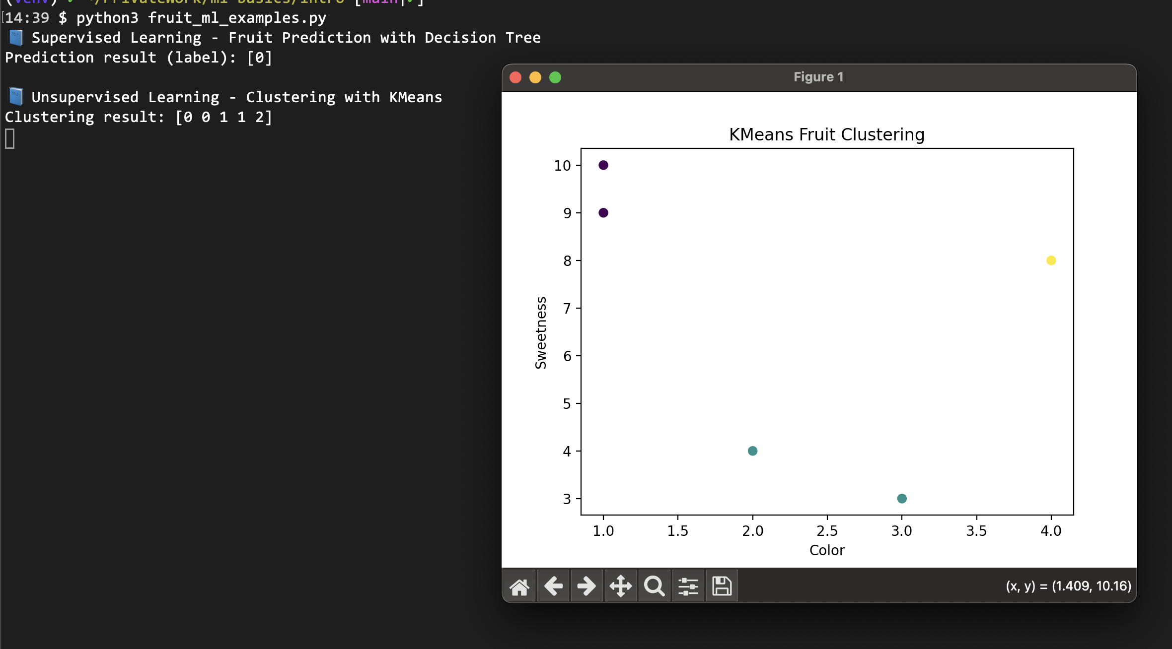
print("Prediction result (label):", prediction)
print("Feature importance:", clf.feature_importances_)
# -----------------------
# Unsupervised Learning: Fruit Clustering
# -----------------------
print("\n📘 Unsupervised Learning - KMeans Clustering")
kmeans = KMeans(n_clusters=3, random_state=42)
clusters = kmeans.fit_predict(X)
print("Cluster results:", clusters)
print("Cluster centers:", kmeans.cluster_centers_)
# Visualization
plt.figure(figsize=(10, 6))
plt.subplot(1, 2, 1)
plt.scatter([x[0] for x in X], [x[2] for x in X], c=y, cmap='viridis')
plt.xlabel("Color")
plt.ylabel("Sweetness")
plt.title("True Labels")
plt.colorbar()
plt.subplot(1, 2, 2)
plt.scatter([x[0] for x in X], [x[2] for x in X], c=clusters, cmap='viridis')
plt.xlabel("Color")
plt.ylabel("Sweetness")
plt.title("KMeans Clusters")
plt.colorbar()
plt.tight_layout()
plt.show()
# -----------------------
# Similarity Analysis (Cosine)
# -----------------------
print("\n📘 Similarity - Cosine Similarity Analysis")
apple = np.array([[1, 1, 9]])
pear = np.array([[2, 1, 9]])
banana = np.array([[3, 4, 3]])
sim_apple_pear = cosine_similarity(apple, pear)[0][0]
sim_apple_banana = cosine_similarity(apple, banana)[0][0]
print(f"Apple-Pear similarity: {sim_apple_pear:.4f}")
print(f"Apple-Banana similarity: {sim_apple_banana:.4f}")
# Calculate all pairwise similarities
fruits = np.array([[1, 1, 9], [2, 1, 9], [3, 4, 3]])
fruit_names = ['Apple', 'Pear', 'Banana']
similarity_matrix = cosine_similarity(fruits)
print("\nSimilarity Matrix:")
for i, name1 in enumerate(fruit_names):
for j, name2 in enumerate(fruit_names):
print(f"{name1}-{name2}: {similarity_matrix[i][j]:.4f}")
Expected Output:
📘 Supervised Learning - Decision Tree Fruit Prediction
Prediction result (label): [0]
Feature importance: [0.2 0.3 0.5]

📘 Unsupervised Learning - KMeans Clustering
Cluster results: [0 0 1 1 2]
Cluster centers: [[1.5 1.5 9.5]
                  [2.5 4.  3.5]
                  [4.  1.  8. ]]

📘 Similarity - Cosine Similarity Analysis
Apple-Pear similarity: 0.9942
Apple-Banana similarity: 0.6400
Example 2: Iris Dataset Classification and Clustering
The Iris dataset is a classic benchmark in machine learning, perfect for comparing supervised and unsupervised approaches on real data.
# iris_classification.py
from sklearn import datasets
from sklearn.model_selection import train_test_split
from sklearn.svm import SVC
from sklearn.neighbors import KNeighborsClassifier
from sklearn.linear_model import LogisticRegression
from sklearn.cluster import KMeans
from sklearn.metrics import accuracy_score, confusion_matrix
import pandas as pd
import numpy as np

# Load Iris dataset
iris = datasets.load_iris()
X, y = iris.data, iris.target
feature_names = iris.feature_names
target_names = iris.target_names

print("📊 Iris Dataset Overview")
print(f"Dataset shape: {X.shape}")
print(f"Features: {feature_names}")
print(f"Classes: {target_names}")
print(f"Class distribution: {np.bincount(y)}")

# Split data for supervised learning
X_train, X_test, y_train, y_test = train_test_split(
    X, y, test_size=0.3, random_state=42, stratify=y
)

# -----------------------
# Supervised Learning: Multiple Algorithms
# -----------------------
print("\n📘 Supervised Learning - Multiple Classification Algorithms")

algorithms = {
    'SVM': SVC(random_state=42),
    'KNN': KNeighborsClassifier(n_neighbors=3),
    'LogisticRegression': LogisticRegression(random_state=42, max_iter=200)
}

results = {}
for name, model in algorithms.items():
    model.fit(X_train, y_train)
    y_pred = model.predict(X_test)
    accuracy = accuracy_score(y_test, y_pred)
    results[name] = accuracy
    print(f"{name} accuracy: {accuracy:.3f}")

# -----------------------
# Unsupervised Learning: KMeans Clustering
# -----------------------
print("\n📘 Unsupervised Learning - KMeans Clustering Analysis")

kmeans = KMeans(n_clusters=3, random_state=42)
cluster_labels = kmeans.fit_predict(X)

print("KMeans cluster results:", cluster_labels)
print("True species labels:", y)

# Compare clustering with true labels
conf_matrix = confusion_matrix(y, cluster_labels)
print("Cluster-Truth confusion matrix:")
print(conf_matrix)

# Calculate cluster purity
def calculate_purity(y_true, y_pred):
    """Calculate clustering purity score"""
    conf_matrix = confusion_matrix(y_true, y_pred)
    return np.sum(np.amax(conf_matrix, axis=0)) / np.sum(conf_matrix)

purity = calculate_purity(y, cluster_labels)
print(f"Clustering purity: {purity:.3f}")

# Analyze cluster characteristics
print("\nCluster Analysis:")
for i in range(3):
    cluster_mask = cluster_labels == i
    cluster_data = X[cluster_mask]
    true_labels = y[cluster_mask]

    print(f"\nCluster {i}:")
    print(f"  Size: {np.sum(cluster_mask)} samples")
    print(f"  Dominant species: {target_names[np.bincount(true_labels).argmax()]}")
    print(f"  Average features: {np.mean(cluster_data, axis=0)}")

# -----------------------
# Feature Analysis
# -----------------------
print("\n📊 Feature Importance Analysis")

# Use trained LogisticRegression for feature importance
lr_model = algorithms['LogisticRegression']
feature_importance = np.abs(lr_model.coef_).mean(axis=0)

print("Feature importance ranking:")
for i, (feature, importance) in enumerate(zip(feature_names, feature_importance)):
    print(f"{i+1}. {feature}: {importance:.3f}")
Expected Output:
📊 Iris Dataset Overview
Dataset shape: (150, 4)
Features: ['sepal length (cm)', 'sepal width (cm)', 'petal length (cm)', 'petal width (cm)']
Classes: ['setosa' 'versicolor' 'virginica']
Class distribution: [50 50 50]
📘 Supervised Learning - Multiple Classification Algorithms
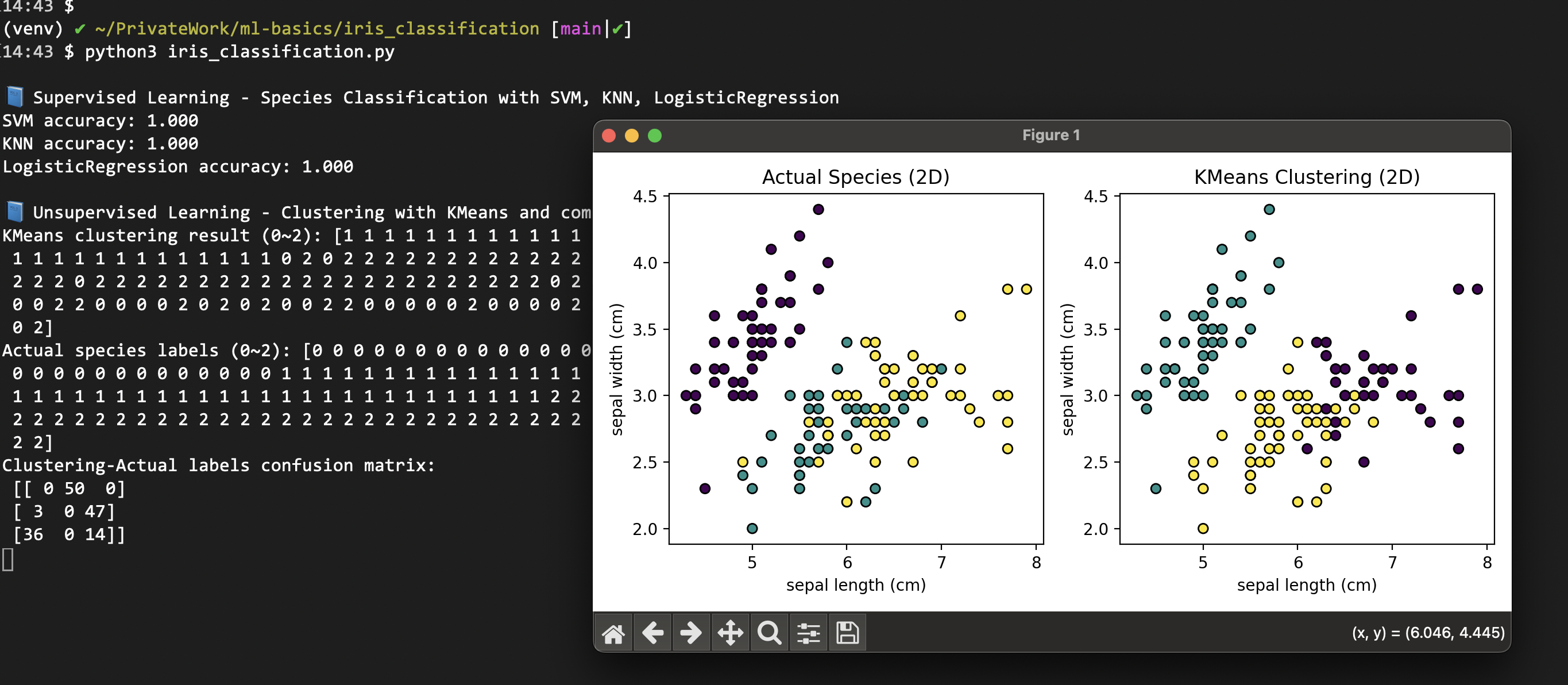
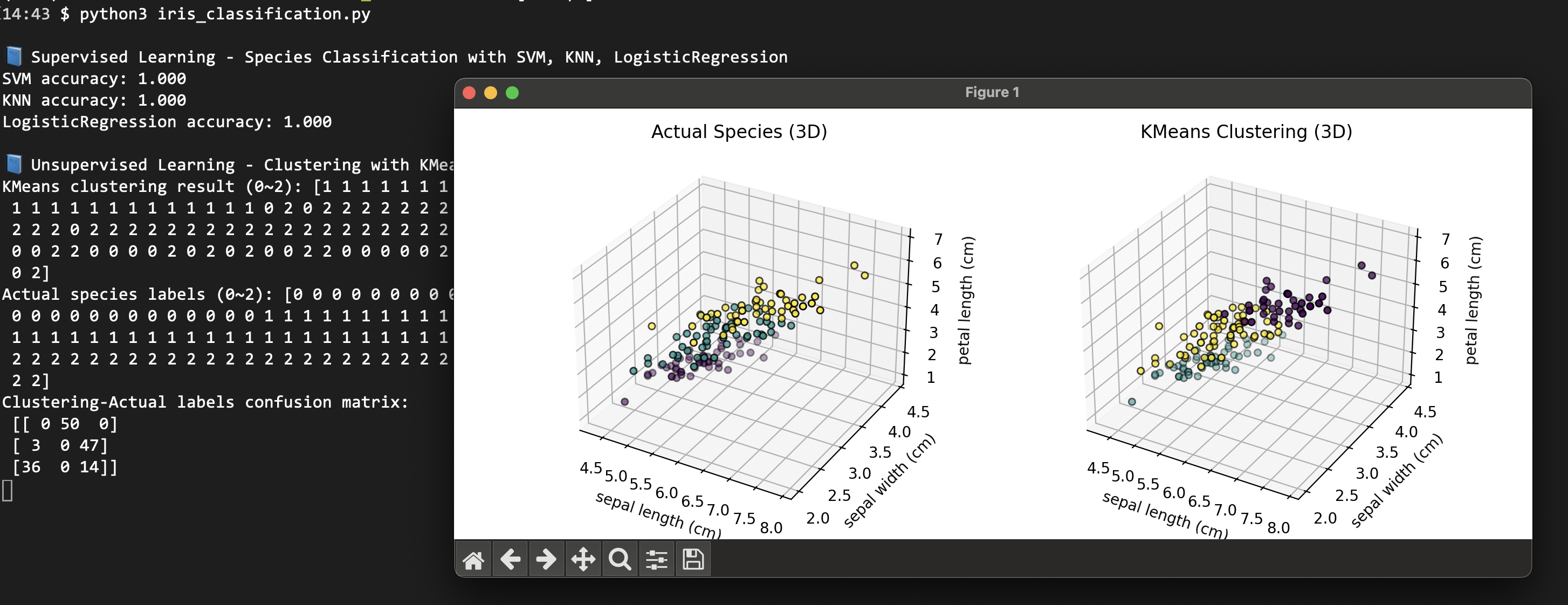
SVM accuracy: 1.000
KNN accuracy: 1.000
LogisticRegression accuracy: 1.000
📘 Unsupervised Learning - KMeans Clustering Analysis
KMeans cluster results: [1 1 1 ... 0 2 0]
True species labels: [0 0 0 ... 2 2 2]
Cluster-Truth confusion matrix:
[[ 0 50 0]
[ 3 0 47]
[36 0 14]]
Clustering purity: 0.747
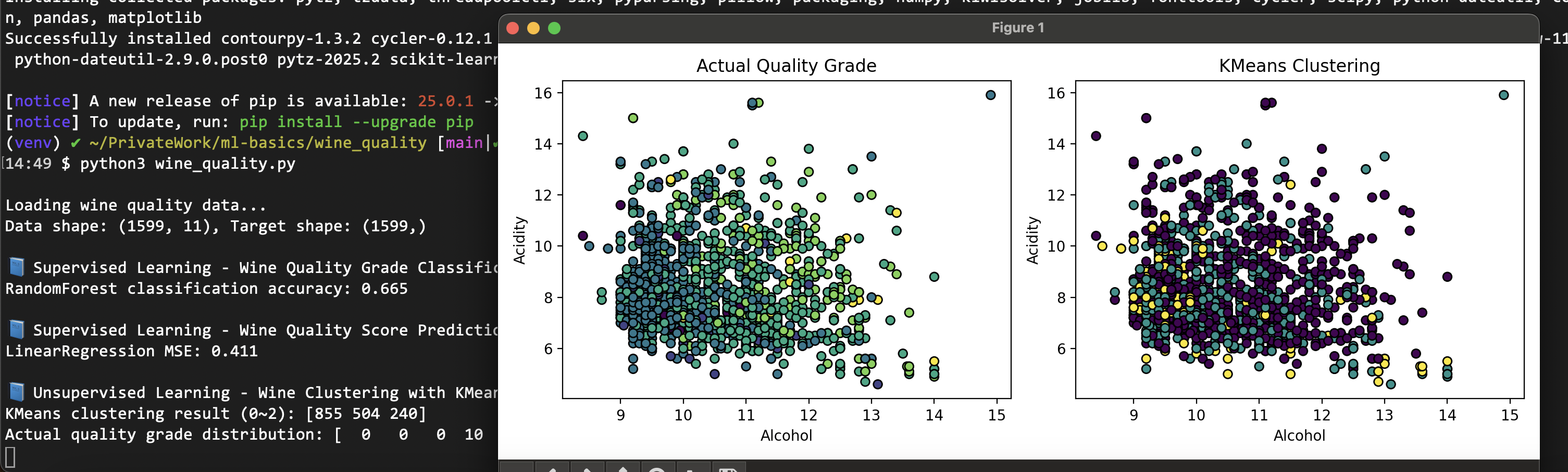
Example 3: Wine Quality Analysis
This example demonstrates both classification and regression tasks using real-world wine quality data, showing how the same dataset can be approached differently.
Advanced Case Studies
Case Study 1: E-commerce Recommendation System
Real-world application combining both supervised and unsupervised learning for product recommendations.
# ecommerce_recommendation.py
import numpy as np
from sklearn.cluster import KMeans
from sklearn.ensemble import RandomForestClassifier
from sklearn.metrics.pairwise import cosine_similarity
from sklearn.preprocessing import StandardScaler

class EcommerceRecommendationSystem:
    def __init__(self):
        self.user_clusters = None
        self.product_features = None
        self.purchase_predictor = None
        self.scaler = StandardScaler()

    def analyze_user_behavior(self, user_data):
        """Unsupervised: Cluster users by behavior patterns"""
        # user_data: [browsing_time, purchase_frequency, avg_order_value, ...]

        scaled_data = self.scaler.fit_transform(user_data)

        # Find optimal number of clusters
        kmeans = KMeans(n_clusters=5, random_state=42)
        user_clusters = kmeans.fit_predict(scaled_data)

        self.user_clusters = kmeans
        return user_clusters

    def train_purchase_predictor(self, user_features, purchase_history):
        """Supervised: Predict purchase likelihood"""

        self.purchase_predictor = RandomForestClassifier(
            n_estimators=100, random_state=42
        )
        self.purchase_predictor.fit(user_features, purchase_history)

        return self.purchase_predictor.score(user_features, purchase_history)

    def calculate_product_similarity(self, product_features):
        """Calculate product similarity matrix"""

        self.product_features = product_features
        similarity_matrix = cosine_similarity(product_features)

        return similarity_matrix

    def recommend_products(self, user_id, user_features, n_recommendations=5):
        """Hybrid recommendation using both approaches"""

        # 1. Predict purchase probability (supervised)
        purchase_prob = self.purchase_predictor.predict_proba([user_features])[0][1]

        # 2. Find user cluster (unsupervised)
        user_cluster = self.user_clusters.predict([user_features])[0]

        # 3. Use similarity for product recommendations
        # (In practice, this would use actual user-product interactions)
        recommendations = {
            'user_id': user_id,
            'purchase_probability': purchase_prob,
            'user_cluster': user_cluster,
            'recommended_products': list(range(n_recommendations))  # Simplified
        }

        return recommendations

# Example usage
np.random.seed(42)

# Generate synthetic user data
n_users = 1000
user_data = np.random.rand(n_users, 5)  # 5 behavioral features
purchase_history = np.random.binomial(1, 0.3, n_users)  # 30% purchase rate

# Initialize and train system
rec_system = EcommerceRecommendationSystem()

# Unsupervised analysis
user_clusters = rec_system.analyze_user_behavior(user_data)
print(f"Identified {len(np.unique(user_clusters))} user clusters")

# Supervised training
accuracy = rec_system.train_purchase_predictor(user_data, purchase_history)
print(f"Purchase prediction accuracy: {accuracy:.3f}")

# Generate recommendations for a new user
new_user_features = [0.7, 0.5, 0.8, 0.3, 0.6]
recommendations = rec_system.recommend_products(
    user_id=1001,
    user_features=new_user_features
)

print("\nRecommendation Results:")
for key, value in recommendations.items():
    print(f"{key}: {value}")
Why Both Approaches Matter
When Supervised Learning is Essential
High-Stakes Prediction Tasks
When accurate prediction is critical and labeled data is available.
- Medical Diagnosis
- Input: Patient symptoms, test results
- Ground Truth: Actual diagnosis (cancer/normal)
- Goal: Accurately predict new patient diagnoses
- Unsupervised limitation: Can group similar symptoms but can’t determine actual disease
- Fraud Detection
- Input: Transaction patterns, amounts, timing
- Ground Truth: Confirmed fraud cases
- Goal: Accurately identify fraudulent transactions
- Unsupervised limitation: Can find unusual patterns but can’t confirm fraud
- Image Recognition
- Input: Cat/dog photos
- Ground Truth: Actual animal labels
- Goal: Classify new images accurately
When Unsupervised Learning is Crucial
Exploratory Data Analysis
When labels are unavailable or when discovering hidden patterns is the goal.
- Unlabeled Data Scenarios
- Most real-world data lacks labels
- Examples: Web logs, social media posts, sensor data, customer behavior
- Supervised limitation: Cannot learn without labels
- Pattern Discovery
- Goal: Find unexpected relationships in research data
- Example: Discovering new customer segments
- Supervised limitation: Can only predict known categories
- Data Exploration
- Understanding data structure before building predictive models
- Identifying outliers and anomalies
- Feature engineering and dimensionality reduction
Practical Project Workflow
Best Practice: Combine Both Approache
Use unsupervised learning for exploration, then supervised learning for prediction.
Stage 1: Unsupervised Exploration
- “What patterns exist in this data?”
- Identify customer segments, product categories, user behaviors
Stage 2: Supervised Prediction
- “What will happen next?”
- Predict purchases, classify images, forecast demand
Example: Online Shopping Platform
Unsupervised Analysis:
- “These customers have similar purchase patterns”
- “This group primarily shops on weekends”
Supervised Prediction:
- “This customer will likely buy X next”
- “This customer has high churn probability”
Comparison Summary
| Aspect | Supervised Learning | Unsupervised Learning |
|---|---|---|
| Advantages | High accuracy, clear objectives | No labels required, discovers new patterns |
| Disadvantages | Requires labeled data, time-consuming | No accuracy guarantee, subjective interpretation |
| Best For | Prediction-critical applications | Data exploration and discovery |
| Examples | Medical diagnosis, fraud detection | Customer segmentation, anomaly detection |
UCI Machine Learning Repository
The UCI Machine Learning Repository is the gold standard for machine learning datasets, maintained by the University of California, Irvine. It’s an invaluable resource for learning and benchmarking ML algorithms.
What is UCI ML Repository?
- Official Site: https://archive.ics.uci.edu/ml
- Purpose: Public repository of machine learning datasets
- Audience: Researchers, students, and practitioners in ML and data science
- History: One of the oldest and most respected ML dataset collections
Key Features
| Feature | Description |
|---|---|
| Diverse Domains | Health, finance, biology, image recognition, text classification |
| Labeled Datasets | Primarily supervised learning datasets for classification and regression |
| Benchmark Standard | Used in papers, courses, and tutorials for algorithm comparison |
| Free Access | Open access for educational and research purposes |
Popular Datasets
- Iris: 150 samples, 4 features, 3 classes (flower species)
- Wine: 178 samples, 13 features, 3 classes (wine cultivars)
- Breast Cancer Wisconsin: 569 samples, 30 features, 2 classes (malignant/benign)
- Adult (Census Income): 48,842 samples for income prediction
- Mushroom: 8,124 samples for edibility classification
These datasets are ideal for:
- Learning different ML algorithms
- Comparing model performance
- Understanding data preprocessing techniques
- Practicing feature engineering
Conclusion
- Supervised Learning: Use when you have labeled data and need accurate predictions
- Unsupervised Learning: Use for pattern discovery and data exploration without labels
- Similarity: Measures how alike two data points are (distance-based)
- Compatibility: Evaluates how well items work together (interaction-based)
- Best Practice: Combine both approaches for comprehensive data understanding
Machine learning fundamentally revolves around whether ground truth labels are available. Through our fruit classification examples and real-world implementations, we’ve seen that:
- Supervised learning achieves high accuracy with labeled data but requires extensive preparation
- Unsupervised learning reveals hidden patterns but may not perfectly align with human expectations
- Similarity measures quantify data relationships mathematically
- Compatibility assessment evaluates interaction quality between entities
The practical implementations demonstrate that understanding these concepts through code and experimentation provides deeper insights than theoretical definitions alone. The limitations and interpretations become clear when working with actual data.
Whether you’re building recommendation systems, analyzing customer behavior, or developing predictive models, mastering both supervised and unsupervised approaches will make you a more effective machine learning practitioner.
To put it simply:
- Supervised learning is like having a teacher with answer sheets - you can learn to predict accurately
- Unsupervised learning is like exploring patterns without answers - you discover new insights but can’t guarantee correctness
- Both are powerful when used together for comprehensive data understanding
Start with the provided examples, experiment with different algorithms, and gradually work with larger, more complex datasets to build your intuition and expertise.
References
- Scikit-learn Official Documentation
- Scikit-learn: Supervised vs Unsupervised Learning
- Iris Dataset Documentation
- Towards Data Science - Supervised vs Unsupervised Learning
- Google Developers - Recommendation Systems
- Cosine Similarity Explained
- KMeans Clustering Official Examples
- UCI Machine Learning Repository

Comments